7.3 AR(1) observed with error

With the addition of \(b\) in front of \(x_{t-1}\) we have an AR(1) process. \[\begin{equation} \begin{gathered} x_{t} = b x_{t-1} + u + w_{t}, \text{ } w_t \sim \,\text{N}(0,q) \\ y_{t} = x_{t} + v_{t}, \text{ } w_t \sim \,\text{N}(0,r) \end{gathered} (\#eq:short-ar1) \end{equation}\]

Create some simulated, non-stationary, AR(1) data:

set.seed(123)
u <- 0.01
r <- 0.1
q <- 0.1
b <- 0.9
TT <- 100
x0 <- 10
xt.ns <- rep(x0, TT)
for (i in 2:TT) xt.ns[i] <- b * xt.ns[i - 1] + u + rnorm(1, 0, 
    sqrt(q))
yt.ns <- xt.ns + rnorm(TT, 0, sqrt(r))

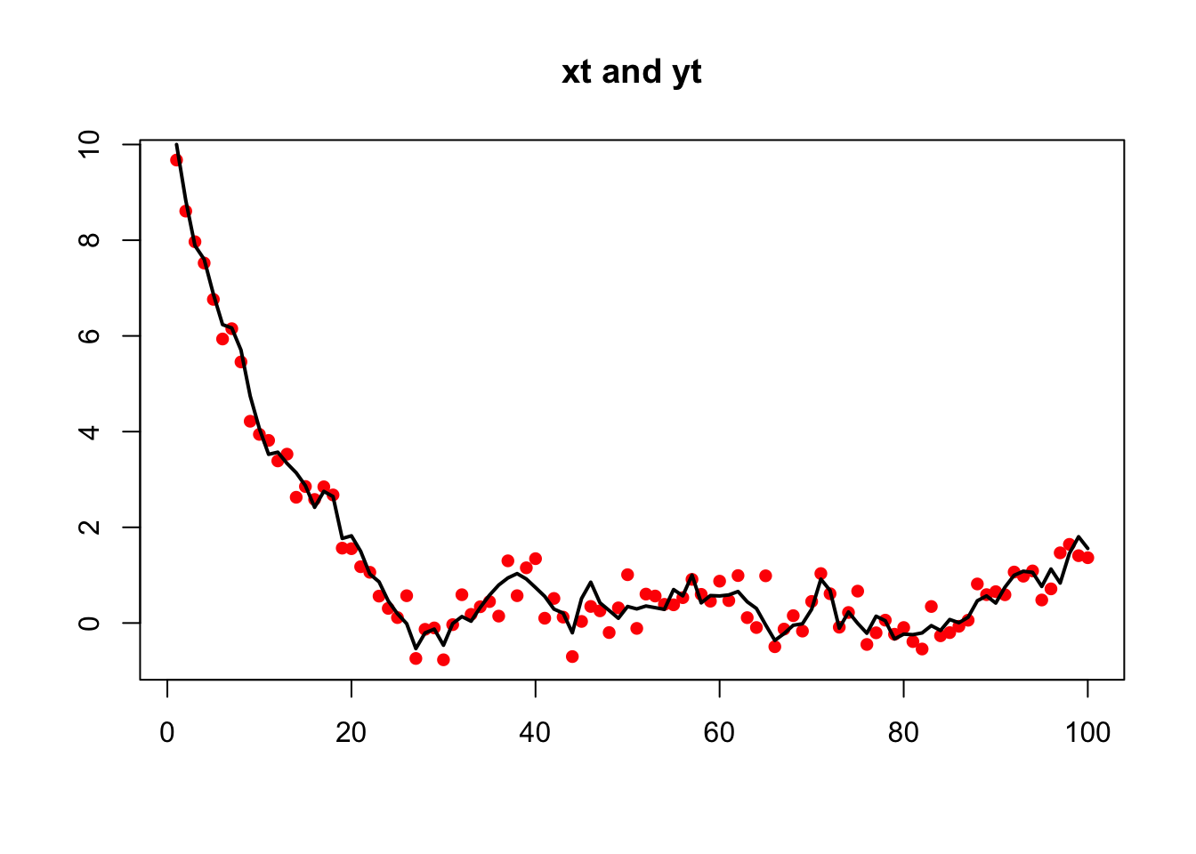
The data were purposefully made to be non-stationary by setting x0 well outside the stationary distribution of \(x\). The EM algorithm in MARSS does not require that the underlying state processes be stationary and it is not necessary to remove the initial non-stationary part of the time-series.

plot(yt.ns, xlab = "", ylab = "", main = "xt and yt", pch = 16, 
    col = "red")
lines(xt.ns, lwd = 2)

fit <- MARSS(yt.ns, model = list(B = matrix("b")))

Success! abstol and log-log tests passed at 24 iterations.
Alert: conv.test.slope.tol is 0.5.
Test with smaller values (<0.1) to ensure convergence.

MARSS fit is
Estimation method: kem 
Convergence test: conv.test.slope.tol = 0.5, abstol = 0.001
Estimation converged in 24 iterations. 
Log-likelihood: -61.67475 
AIC: 133.3495   AICc: 133.9878   
 
      Estimate
R.R     0.1075
B.b     0.9042
U.U     0.0346
Q.Q     0.0535
x0.x0  10.6409
Initial states (x0) defined at t=0

Standard errors have not been calculated. 
Use MARSSparamCIs to compute CIs and bias estimates.

We could also simulate AR(1) data with stats::arima.sim() however this will produce stationary data:

xt.s <- arima.sim(n = TT, model = list(ar = b), sd = sqrt(q))
yt.s <- xt.s + rnorm(TT, 0, sqrt(r))
yt.s <- as.vector(yt.s)
xt.s <- as.vector(xt.s)

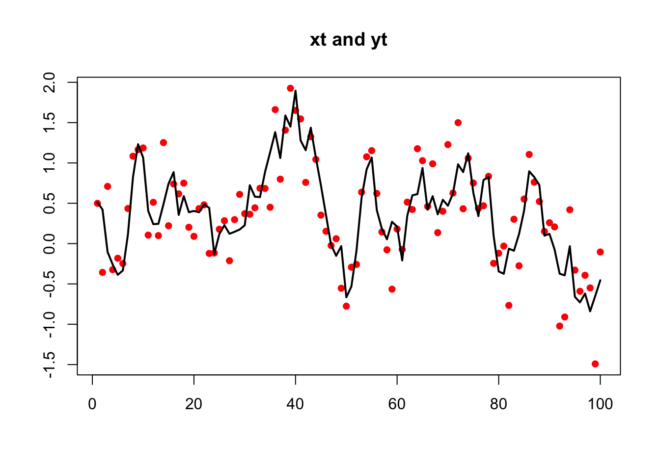
These stationary data can be fit as before but the data must be a matrix with time across the columns not a ts object. If you pass in a vector, MARSS() will convert that to a matrix with one row.

plot(yt.s, xlab = "", ylab = "", main = "xt and yt", pch = 16, 
    col = "red", type = "p")
lines(xt.s, lwd = 2)

fit <- MARSS(yt.s, model = list(B = matrix("b")))

Success! abstol and log-log tests passed at 27 iterations.
Alert: conv.test.slope.tol is 0.5.
Test with smaller values (<0.1) to ensure convergence.

MARSS fit is
Estimation method: kem 
Convergence test: conv.test.slope.tol = 0.5, abstol = 0.001
Estimation converged in 27 iterations. 
Log-likelihood: -74.40797 
AIC: 158.8159   AICc: 159.4542   
 
      Estimate
R.R     0.1064
B.b     0.7884
U.U     0.0735
Q.Q     0.1142
x0.x0   0.2825
Initial states (x0) defined at t=0

Standard errors have not been calculated. 
Use MARSSparamCIs to compute CIs and bias estimates.

Note that \(u\) is estimated however arima.sim() does not include a \(u\). We can set \(u\) to zero if we happened to know that it was zero.

fit <- MARSS(yt.s, model = list(B = matrix("b"), U = matrix(0)))

Success! abstol and log-log tests passed at 16 iterations.
Alert: conv.test.slope.tol is 0.5.
Test with smaller values (<0.1) to ensure convergence.

MARSS fit is
Estimation method: kem 
Convergence test: conv.test.slope.tol = 0.5, abstol = 0.001
Estimation converged in 16 iterations. 
Log-likelihood: -75.80277 
AIC: 159.6055   AICc: 160.0266   
 
      Estimate
R.R      0.117
B.b      0.874
Q.Q      0.100
x0.x0    0.339
Initial states (x0) defined at t=0

Standard errors have not been calculated. 
Use MARSSparamCIs to compute CIs and bias estimates.

If we know \(r\) (or \(q\)), we could set those too:

fit <- MARSS(yt.s, model = list(B = matrix("b"), U = matrix(0), 
    R = matrix(r)))

Success! abstol and log-log tests passed at 18 iterations.
Alert: conv.test.slope.tol is 0.5.
Test with smaller values (<0.1) to ensure convergence.

MARSS fit is
Estimation method: kem 
Convergence test: conv.test.slope.tol = 0.5, abstol = 0.001
Estimation converged in 18 iterations. 
Log-likelihood: -75.88583 
AIC: 157.7717   AICc: 158.0217   
 
      Estimate
B.b      0.859
Q.Q      0.114
x0.x0    0.370
Initial states (x0) defined at t=0

Standard errors have not been calculated. 
Use MARSSparamCIs to compute CIs and bias estimates.

We can fit to just the \(x\) data, an AR(1) with no error, by setting \(r\) to zero: If we know \(r\) (or \(q\)), we could set those too:

fit <- MARSS(xt.s, model = list(B = matrix("b"), U = matrix(0), 
    R = matrix(0)))

Success! algorithm run for 15 iterations. abstol and log-log tests passed.
Alert: conv.test.slope.tol is 0.5.
Test with smaller values (<0.1) to ensure convergence.

MARSS fit is
Estimation method: kem 
Convergence test: conv.test.slope.tol = 0.5, abstol = 0.001
Algorithm ran 15 (=minit) iterations and convergence was reached. 
Log-likelihood: -26.9401 
AIC: 59.8802   AICc: 60.1302   
 
      Estimate
B.b      0.883
Q.Q      0.100
x0.x0    0.578
Initial states (x0) defined at t=0

Standard errors have not been calculated. 
Use MARSSparamCIs to compute CIs and bias estimates.

We can fit xt.s with arima() also. The results will be similar but not identical because arima()’s algorithm assumes the data come from a stationary process and the initial conditions are treated differently.

arima(xt.s, order = c(1, 0, 0), include.mean = FALSE, method = "ML")

Call:
arima(x = xt.s, order = c(1, 0, 0), include.mean = FALSE, method = "ML")

Coefficients:
         ar1
      0.8793
s.e.  0.0454

sigma^2 estimated as 0.1009:  log likelihood = -27.98,  aic = 59.96

If we try fitting the non-stationary data with arima(), the estimates will be poor since arima() assumes stationary data:

arima(xt.ns, order = c(1, 0, 0), include.mean = FALSE, method = "ML")

Call:
arima(x = xt.ns, order = c(1, 0, 0), include.mean = FALSE, method = "ML")

Coefficients:
         ar1
      0.9985
s.e.  0.0021

sigma^2 estimated as 0.1348:  log likelihood = -44.59,  aic = 93.19