7.8 Flat level model

For the next examples, we will use the Nile river flow from 1871 to 1970, a data set in the datasets package.

nile <- as.vector(datasets::Nile)
year <- as.vector(time(Nile))

The first model we will fit is a flat level model:

\[\begin{equation} y_t = a+v_t, \text{ } v_t \sim \,\text{N}(0,r) \tag{7.12} \end{equation}\] where \(y_t\) is the river flow volume at year \(t\) and \(a\) is some constant average flow level (notice it has no \(t\) subscript).

To fit this model with MARSS, we explicitly show all the MARSS parameters. \[\begin{equation} \begin{gathered} x_t = 1 \times x_{t-1}+ 0 + w_t, \text{ } w_t \sim \,\text{N}(0,0) \\ y_t = 0 \times x_t + a + v_t, \text{ } v_t \sim \,\text{N}(0,r) \\ x_0 = 0 \end{gathered} \tag{7.13} \end{equation}\]

The model list and fit for this equation is

mod.list1 <- list(Z = matrix(0), A = matrix("a"), R = matrix("r"), 
    B = matrix(1), U = matrix(0), Q = matrix(0), x0 = matrix(0))
fit1 <- MARSS(nile, model = mod.list1)

Success! abstol and log-log tests passed at 16 iterations.
Alert: conv.test.slope.tol is 0.5.
Test with smaller values (<0.1) to ensure convergence.

MARSS fit is
Estimation method: kem 
Convergence test: conv.test.slope.tol = 0.5, abstol = 0.001
Estimation converged in 16 iterations. 
Log-likelihood: -654.5157 
AIC: 1313.031   AICc: 1313.155   
 
    Estimate
A.a      919
R.r    28352
Initial states (x0) defined at t=0

Standard errors have not been calculated. 
Use MARSSparamCIs to compute CIs and bias estimates.

MARSS includes the state process \(x_t\) but we are setting \(\mathbf{Z}\) to zero so that \(x_t\) does not appear in our observation model. We need to fix all the state parameters to zero so that the algorithm doesn’t ``chase its tail’’ trying to fit \(x_t\) to the data.

An equivalent way to write this model is to use \(x_t\) as the average flow level and make it be a constant level by setting \(q=0\). The average flow appears as the \(x_0\) parameter. In MARSS form, this model is:

\[\begin{equation} \begin{gathered} x_t = 1 \times x_{t-1}+ 0 + w_t \text{ where } w_t \sim \,\text{N}(0,0) \\ y_t = 1 \times x_t + 0 + v_t \text{ where } v_t \sim \,\text{N}(0,r) \\ x_0 = a \end{gathered} \tag{7.14} \end{equation}\]

The model list and fit for this equation is

mod.list2 <- list(Z = matrix(1), A = matrix(0), R = matrix("r"), 
    B = matrix(1), U = matrix(0), Q = matrix(0), x0 = matrix("a"))
fit2 <- MARSS(nile, model = mod.list2)

Success! algorithm run for 15 iterations. abstol and log-log tests passed.
Alert: conv.test.slope.tol is 0.5.
Test with smaller values (<0.1) to ensure convergence.

MARSS fit is
Estimation method: kem 
Convergence test: conv.test.slope.tol = 0.5, abstol = 0.001
Algorithm ran 15 (=minit) iterations and convergence was reached. 
Log-likelihood: -654.5157 
AIC: 1313.031   AICc: 1313.155   
 
     Estimate
R.r     28352
x0.a      919
Initial states (x0) defined at t=0

Standard errors have not been calculated. 
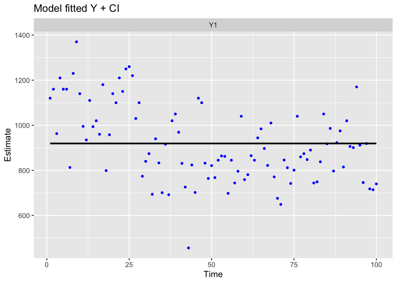
Use MARSSparamCIs to compute CIs and bias estimates.

The results are the same. We just formatted the model in different ways. We can plot the fitted model against the Nile river flow (blue dots) using autoplot().

ggplot2::autoplot(fit2, plot.type = "model.ytT")