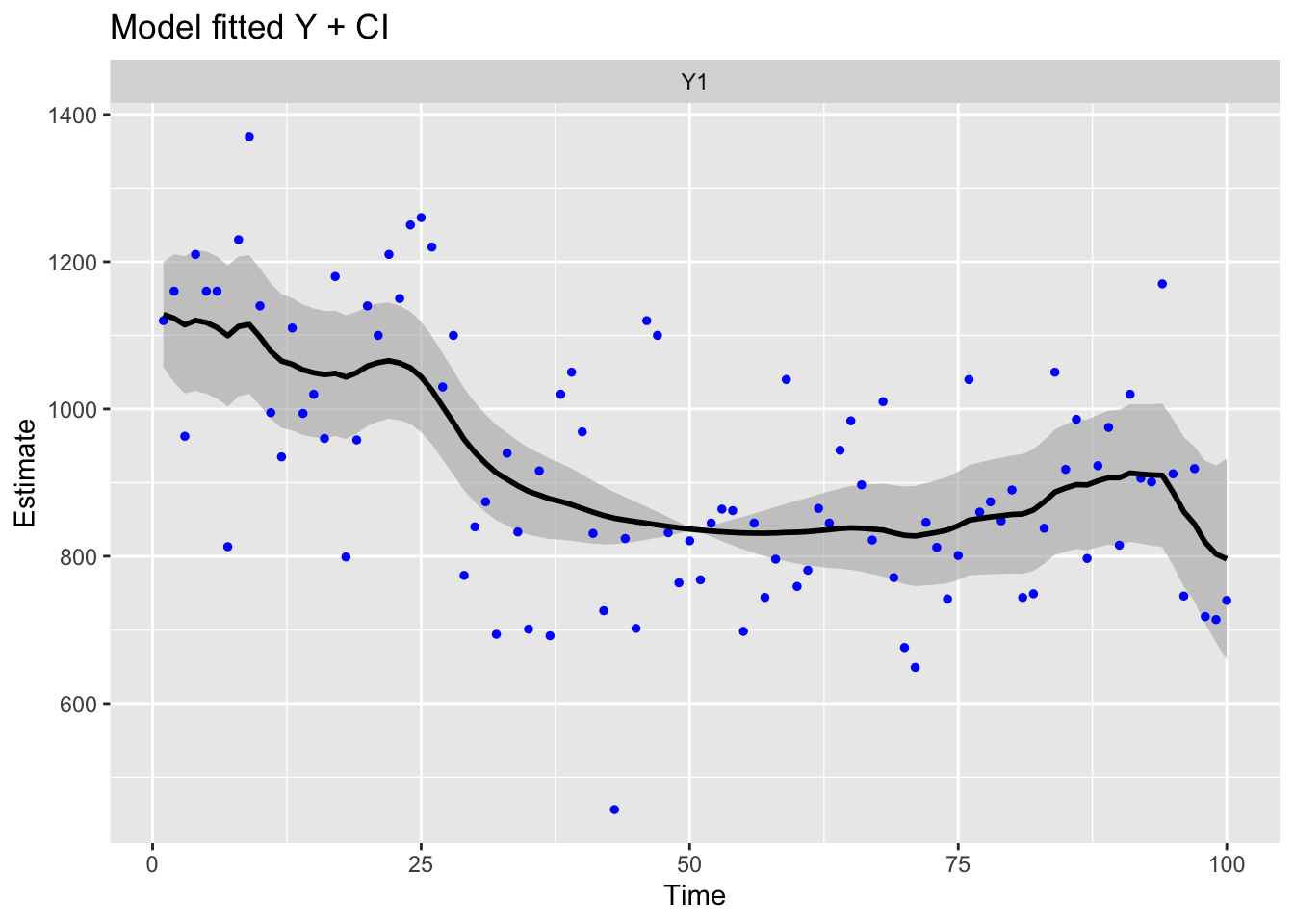
7.11 Stochastic slope model

We can also model the \(\beta\) as a random walk:

\[\begin{equation} \begin{gathered} \beta_t = \beta_{t-1}+w_t, \text{ } w_t \sim \,\text{N}(0,q) \\ y_t = a + \beta_t t + v_t, \text{} v_t \sim \,\text{N}(0,r) \\ x_0 = \pi \end{gathered} \tag{7.19} \end{equation}\]

The \(\beta_t\) is model with \(x_t\). With all the MARSS parameters shown, the model is: \[\begin{equation} \begin{gathered} x_t = 1 \times x_{t-1}+ 0 + w_t, \text{ } w_t \sim \,\text{N}(0,q) \\ y_t = t \times x_t + a + v_t, \text{ } v_t \sim \,\text{N}(0,r) \\ x_0 = \pi \end{gathered} \tag{7.20} \end{equation}\] The trick here is to recognize that \(\mathbf{Z}_t\), the matrix in front of \(\mathbf{x}_t\) in the \(\mathbf{y}_t\) equation, can be time-varying and can be fixed. In a time-varying matrix in MARSS, the time element is in the 3rd dimension. We are going to fix \(\mathbf{Z}[1,1,t] = t\), where \(t\) is year-mean(year). \(\mathbf{Z}\) is a \(1 \times 1 \times 100\) array. Demeaning the covariate stablizes the fitting. Try without demeaning to see the difference.

The model is specified as a list as follows.

Z <- array(0, dim = c(1, 1, length(nile)))
Z[1, 1, ] <- year - mean(year)
mod.list = list(Z = Z, A = matrix("a"), R = matrix("r"), B = matrix(1), 
    U = matrix(0), Q = matrix("q"), x0 = matrix("pi"))
fit1 <- MARSS(nile, model = mod.list, silent = TRUE)
fit2 <- MARSS(nile, model = mod.list, inits = fit1, method = "BFGS")

Success! Converged in 13 iterations.
Function MARSSkfas used for likelihood calculation.

MARSS fit is
Estimation method: BFGS 
Estimation converged in 13 iterations. 
Log-likelihood: -636.6226 
AIC: 1281.245   AICc: 1281.666   
 
       Estimate
A.a     836.164
R.r   16835.484
Q.q       0.749
x0.pi    -5.905
Initial states (x0) defined at t=0

Standard errors have not been calculated. 
Use MARSSparamCIs to compute CIs and bias estimates.

ggplot2::autoplot(fit2, plot.type = "model.ytT")