8.4 Trend observed with AR(1) error

So far we have been assuming that the observations errors, \(\mathbf{v}_t\), are temporally independent. Let’s assume 3 observations of one underlying trend but assume the observations have AR(1) errors. We’ll assume that the variance of those error is correlated across the first 2 time series and they have the same level of autocorrelation (\(b\)). We’ll treat the 3rd time series as independent.

To do this, we need to move the observation errors into the \(\mathbf{x}\) part of the MARSS model and we need to add the \(\mathbf{B}\) matrix for the AR(1) feature. Notice that the \(\mathbf{y}\) equation does not have \(\mathbf{v}_t\) since the observation errors are specified in the \(\mathbf{x}\) part of the equation and are flowing from \(\mathbf{x}\) to \(\mathbf{y}\) via \(\mathbf{Z}\). \[\begin{equation} \begin{gathered} \begin{bmatrix}x_1\\x_2\\x_3\\x_4\end{bmatrix}_t = \begin{bmatrix} 1&0&0&0\\ 0&b_1&0&0\\ 0&0&b_1&0\\ 0&0&0&b_2\\ \end{bmatrix} \begin{bmatrix}x_1\\x_2\\x_3\\x_4\end{bmatrix}_{t-1} + \begin{bmatrix}w_1\\ w_2\\ w_3 \\ w_4\end{bmatrix}, \textrm{ } \mathbf{w}_t \sim \,\text{MVN}\begin{pmatrix} \begin{bmatrix}0\\0\\0\end{bmatrix}, \begin{bmatrix} q_1&0&0&0\\ 0&q_2&c&0\\ 0&c&q_3&0\\ 0&0&0&q_4\end{bmatrix} \end{pmatrix}\\ \begin{bmatrix}y_1\\y_2\\y_3\end{bmatrix}_t = \begin{bmatrix} 1&1&0&0\\ 1&0&1&0\\ 1&0&0&1\end{bmatrix} \begin{bmatrix}x_1\\x_2\\x_3\\x_4\end{bmatrix}_t + \begin{bmatrix}0\\a_2\\a_3\end{bmatrix} \end{gathered} \tag{8.5} \end{equation}\]

Create set up the model.

Z <- matrix(0, 3, 4)
Z[, 1] <- 1
Z[, 2:4] <- diag(1, 3)
R <- U <- A <- "zero"
Q <- matrix(list(0), 4, 4)
diag(Q) <- paste0("q", 1:4)
Q[2, 3] <- Q[3, 2] <- "c"

Print out the Q to make sure it matches our equation.

Q

     [,1] [,2] [,3] [,4]
[1,] "q1" 0    0    0   
[2,] 0    "q2" "c"  0   
[3,] 0    "c"  "q3" 0   
[4,] 0    0    0    "q4"

Fit with MARSS():

yt <- t(harborSealWA)[c("EBays", "SJI", "PSnd"), ]
fit <- MARSS(yt, model = list(R = R, Z = Z, Q = Q, U = U, A = A), 
    inits = list(x0 = matrix(0, 4, 1)))

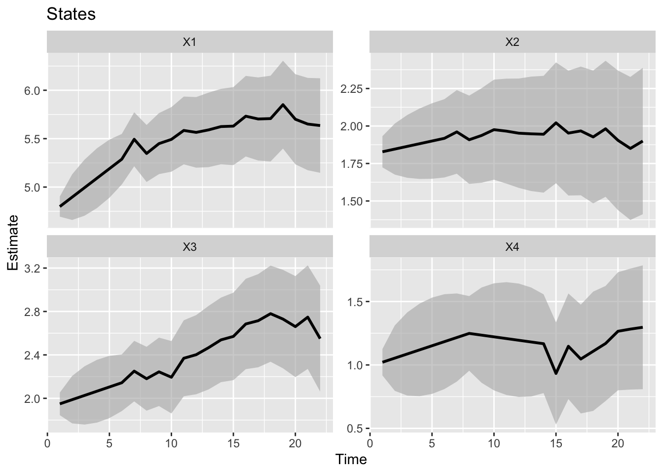
Estimated states. The first one is the trend and the next 3 are the AR(1) errors. If your goal was to estimate the underlying signal, then the plot for X1 is what you want and has the confidence intervals that you want.

ggplot2::autoplot(fit, plot.type = "xtT")

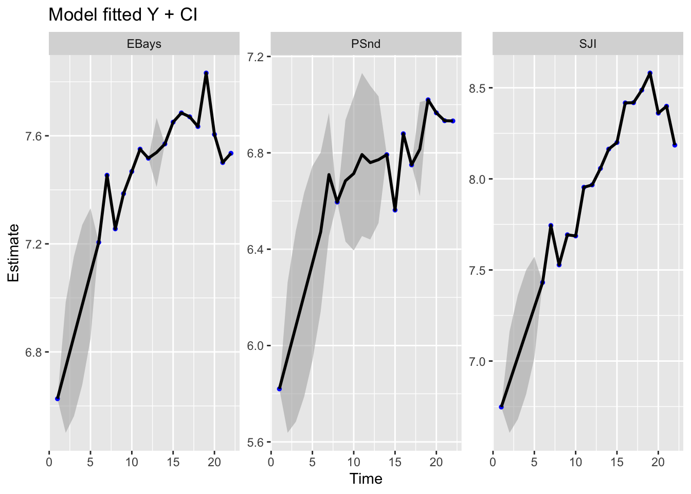
If on the otherhand, you wanted estimates of the numbers in each region then sadly the model fit plots are not what you want. Since \(\mathbf{R}\) was set to 0, the model fits will exactly fit the data. You would need to write a custom function for the expected value of \(\mathbf{y}\) and its variance. The expected value is just the estimated first state (\(x_1\)) plus the corresponding \(a\) term. But the variance would need to computed using the variances of states 2 to 4 (the AR(1) errors).

ggplot2::autoplot(fit, plot.type = "model.ytT")