8.6 Linear constraints

Your model can have simple linear constraints within all the parameters except \(\mathbf{Q}\), \(\mathbf{R}\) and \(\boldsymbol{\Lambda}\). For example \(1+2a-3b\) is a linear constraint. When entering this value for you matrix, you specify this as “1+2a+-3b”@. NOTE: \(+\)’s join parts so use "+-3*b" to specify \(-3b\). Anything after * is a parameter. So 1*1 has a parameter called "1". Example, let’s specify the following \(\mathbf{B}\), \(\mathbf{Q}\) and \(\mathbf{Z}\) matrices: \[\begin{equation*} \mathbf{U} = \begin{bmatrix}u-0.1\\ u+0.1\end{bmatrix}\quad \mathbf{Q} = \begin{bmatrix}q_{11}&0\\ 0.01&0\end{bmatrix}\quad \mathbf{Z} = \begin{bmatrix}z_1-z_2&2z_1\\ 0&z_1\\ z_2&0 \\ 0&z_3 \\ 0&1+z_3\end{bmatrix} \end{equation*}\]

This would be specified as (notice "1*z1+-1*z2" for \(z_1-z_2\)):

U <- matrix(list("-0.1+1*u", "0.1+1*u"), 2, 1)
Q <- matrix(list("q11", 0, 0, 0.01), 2, 2)
Z <- matrix(list("1*z1+-1*z2", 0, "z2", 0, 0, "2*z1", "z1", 0, 
    "z3", "1+z3"), 5, 2)

We need to fix \(\mathbf{A}\) if \(\mathbf{Z}\) is estimated.

yt <- t(harborSealWA)[2:6, ]
fit <- MARSS(yt, model = list(Z = Z, Q = Q, U = U, A = "zero"))

Success! abstol and log-log tests passed at 374 iterations.
Alert: conv.test.slope.tol is 0.5.
Test with smaller values (<0.1) to ensure convergence.

MARSS fit is
Estimation method: kem 
Convergence test: conv.test.slope.tol = 0.5, abstol = 0.001
Estimation converged in 374 iterations. 
Log-likelihood: -129.771 
AIC: 275.5421   AICc: 277.8647   
 
       Estimate
Z.z1     2.9071
Z.z2    11.5822
Z.z3     2.3829
R.diag   1.1864
U.u     -0.0333
Q.q11    0.0291
x0.X1    0.7627
x0.X2    1.9489
Initial states (x0) defined at t=0

Standard errors have not been calculated. 
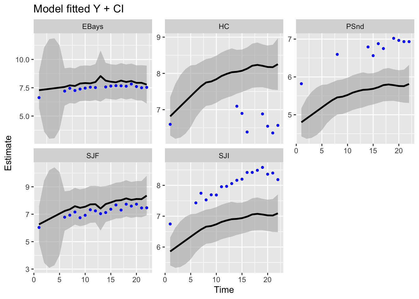
Use MARSSparamCIs to compute CIs and bias estimates.

This is a toy example and cannot fit the data.

ggplot2::autoplot(fit, plot.type = "model.ytT")