7.9 Linear trend model

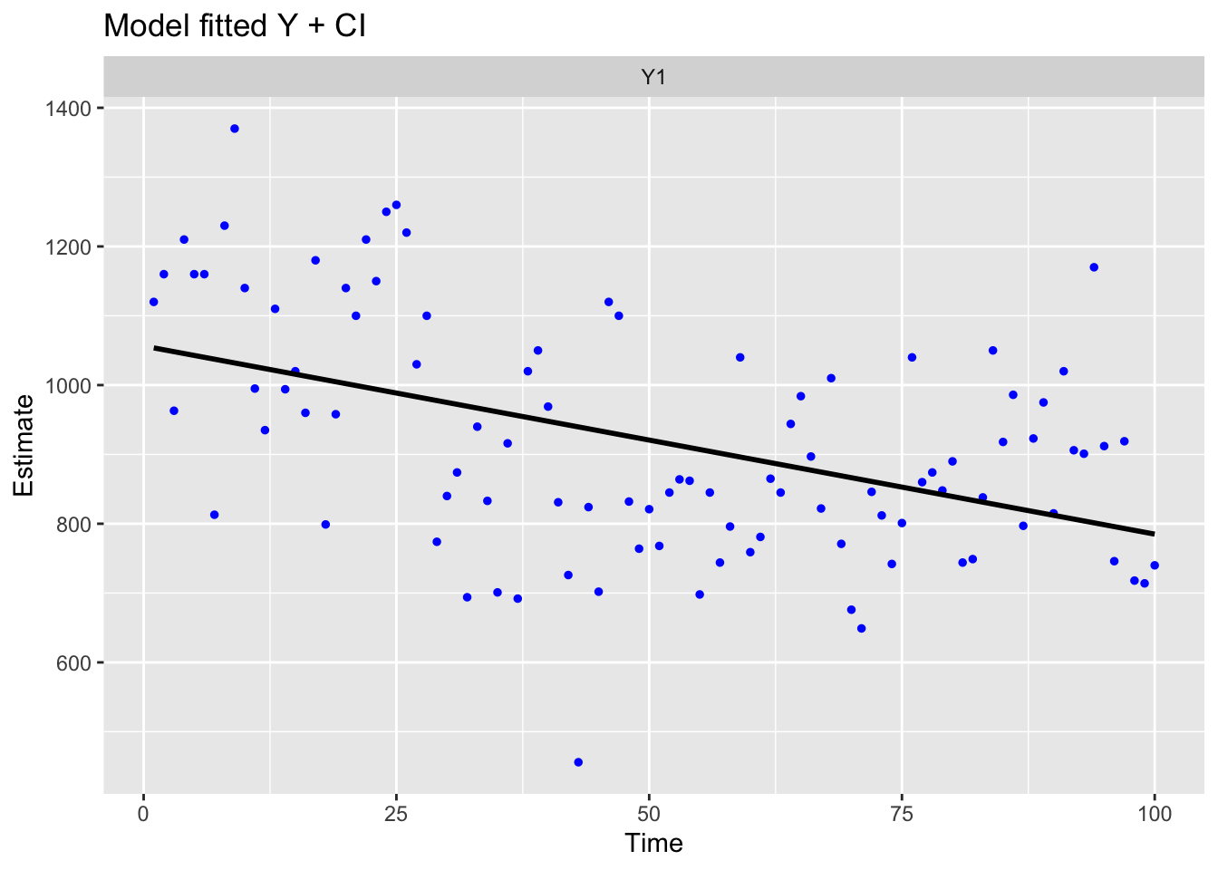
Looking at the data, we might expect that a declining average river flow would be better. In MARSS form, that model would be: \[\begin{equation} \begin{gathered} x_t = 1 \times x_{t-1}+ 0 + w_t, \text{ } w_t \sim \,\text{N}(0,0) \\ y_t = 0 \times x_t + a + \beta t + v_t, \text{ } v_t \sim \,\text{N}(0,r) \\ x_0 = 0 \end{gathered} \tag{7.15} \end{equation}\] where \(t\) is the year and \(u\) is the average per-year decline in river flow volume.

The model list and fit for this equation is

mod.list1 <- list(Z = matrix(0), A = matrix("a"), R = matrix("r"), 
    D = matrix("beta"), d = matrix(1:100, nrow = 1), B = matrix(1), 
    U = matrix(0), Q = matrix(0), x0 = matrix(0))
fit1 <- MARSS(nile, model = mod.list1)

Success! algorithm run for 15 iterations. abstol and log-log tests passed.
Alert: conv.test.slope.tol is 0.5.
Test with smaller values (<0.1) to ensure convergence.

MARSS fit is
Estimation method: kem 
Convergence test: conv.test.slope.tol = 0.5, abstol = 0.001
Algorithm ran 15 (=minit) iterations and convergence was reached. 
Log-likelihood: -642.3147 
AIC: 1290.629   AICc: 1290.879   
 
       Estimate
A.a     1056.42
R.r    22212.64
D.beta    -2.71
Initial states (x0) defined at t=0

Standard errors have not been calculated. 
Use MARSSparamCIs to compute CIs and bias estimates.

We can also write this model as follows by modeling the trend with \(x_t\): \[\begin{equation} \begin{gathered} x_t = 1 \times x_{t-1} + u + w_t, \text{ } w_t \sim \,\text{N}(0,0) \\ y_t = 1 \times x_t + 0 + v_t, \text{ } v_t \sim \,\text{N}(0,r) \\ x_0 = a \end{gathered} \tag{7.16} \end{equation}\]

The model is specified as a list as follows. To fit, we need to force the algorithm to run a bit longer as it is showing convergence a bit early.

mod.list2 = list(Z = matrix(1), A = matrix(0), R = matrix("r"), 
    B = matrix(1), U = matrix("u"), Q = matrix(0), x0 = matrix("a"))
fit2 <- MARSS(nile, model = mod.list2, control = list(minit = 30))

Success! algorithm run for 30 iterations. abstol and log-log tests passed.
Alert: conv.test.slope.tol is 0.5.
Test with smaller values (<0.1) to ensure convergence.

MARSS fit is
Estimation method: kem 
Convergence test: conv.test.slope.tol = 0.5, abstol = 0.001
Algorithm ran 30 (=minit) iterations and convergence was reached. 
Log-likelihood: -642.3147 
AIC: 1290.629   AICc: 1290.879   
 
     Estimate
R.r  22212.64
U.u     -2.71
x0.a  1056.37
Initial states (x0) defined at t=0

Standard errors have not been calculated. 
Use MARSSparamCIs to compute CIs and bias estimates.

The fits are the same with either formulation of the model as long as we force the algorithm to run longer for the second form.

ggplot2::autoplot(fit2, plot.type = "model.ytT")