7.10 Stochastic level model

We will now model the average river flow at year \(t\) as a random walk, specifically an autoregressive process which means that average river flow at year \(t\) is a function of average river flow in year \(t-1\).

\[\begin{equation} \begin{gathered} x_t = x_{t-1}+w_t, \text{ } w_t \sim \,\text{N}(0,q) \\ y_t = x_t+v_t, \text{ } v_t \sim \,\text{N}(0,r) \\ x_0 = \pi \end{gathered} \tag{7.17} \end{equation}\]

With all the MARSS parameters shown, the model is: \[\begin{equation} \begin{gathered} x_t = 1 \times x_{t-1}+ 0 + w_t, \text{ } w_t \sim \,\text{N}(0,q) \\ y_t = 1 \times x_t + 0 + v_t, \text{ } v_t \sim \,\text{N}(0,r) \\ x_0 = \pi \end{gathered} \tag{7.18} \end{equation}\]

The model is specified as a list as follows. We can use the BFGS algorithm to ‘polish’ off the fit and get closer to the MLE. Why not just start with BFGS? First, it happens to take a long long time to fit and more importantly, the BFGS algorith is sensitive to starting conditions and can catostrophically fail. In this case, it is slow but works fine. For some models, it does work better (faster and stable), but using the EM algorithm to get decent starting conditions for the BFGS algorithm is a common fitting strategy.

mod.list = list(Z = matrix(1), A = matrix(0), R = matrix("r"), 
    B = matrix(1), U = matrix(0), Q = matrix("q"), x0 = matrix("pi"))
fit1 <- MARSS(nile, model = mod.list, silent = TRUE)
fit2 <- MARSS(nile, model = mod.list, inits = fit1, method = "BFGS")

Success! Converged in 12 iterations.
Function MARSSkfas used for likelihood calculation.

MARSS fit is
Estimation method: BFGS 
Estimation converged in 12 iterations. 
Log-likelihood: -637.7451 
AIC: 1281.49   AICc: 1281.74   
 
      Estimate
R.r      15337
Q.q       1218
x0.pi     1112
Initial states (x0) defined at t=0

Standard errors have not been calculated. 
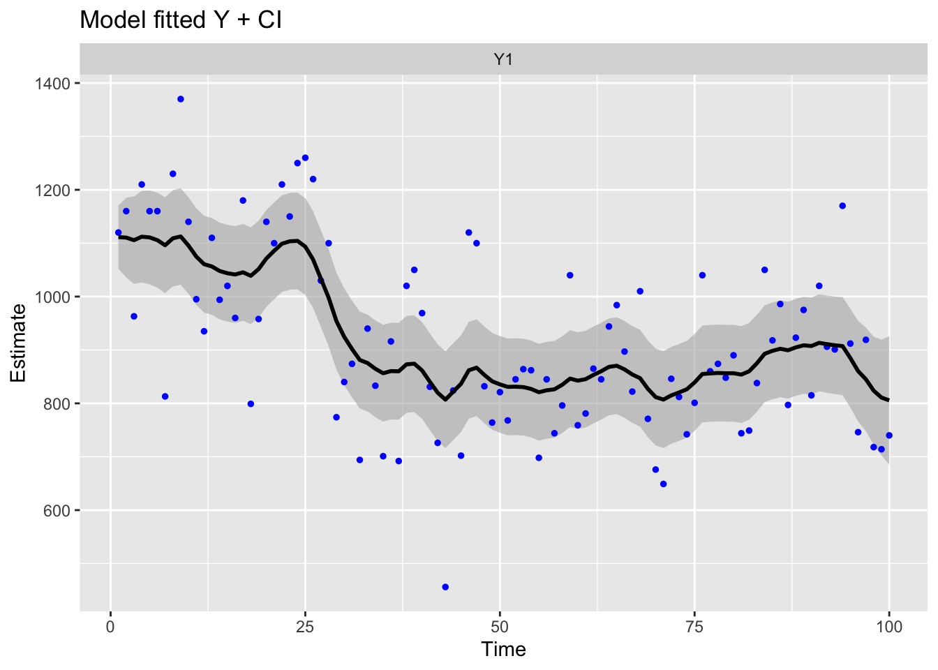
Use MARSSparamCIs to compute CIs and bias estimates.

ggplot2::autoplot(fit2, plot.type = "model.ytT")

This is the same model fit in Koopman, Shephard, and Doornik (1999) (p. 148) except that we estimate \(x_1\) as parameter rather than specifying \(x_1\) via a diffuse prior. As a result, the log-likelihood value and \(\mathbf{R}\) and \(\mathbf{Q}\) are a little different than in Koopman, Shephard, and Doornik (1999).

We can fit the Koopman model with stats::StructTS(). The estimates are slightly different since the initial conditions are treated differently.

fit.ts <- stats::StructTS(nile, type = "level")
fit.ts

Call:
stats::StructTS(x = nile, type = "level")

Variances:
  level  epsilon  
   1469    15099  

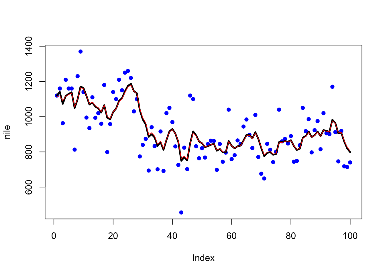
The fitted values returned by fitted() applied to a StructTS object are different than that returned by fitted() applied to a marssMLE object. The former returns \(\hat{y}\) conditioned on the data up to time \(t\), while the latter returns the \(\hat{y}\) conditioned on all the data. If you want to compare use:

plot(nile, type = "p", pch = 16, col = "blue")
lines(fitted(fit.ts), col = "black", lwd = 3)
lines(MARSSkfss(fit2)$xtt[1, ], col = "red", lwd = 1)

The black line is the StrucTS() fit and the red line is the equivalent MARSS() fit.