7.4 Linear regression (LR)

A simple linear regression of one covariate is written:

\[\begin{equation} y_{t} = \alpha + \beta \, d_t + v_{t}, \text{ } w_t \sim \,\text{N}(0,q) \tag{7.5} \end{equation}\]

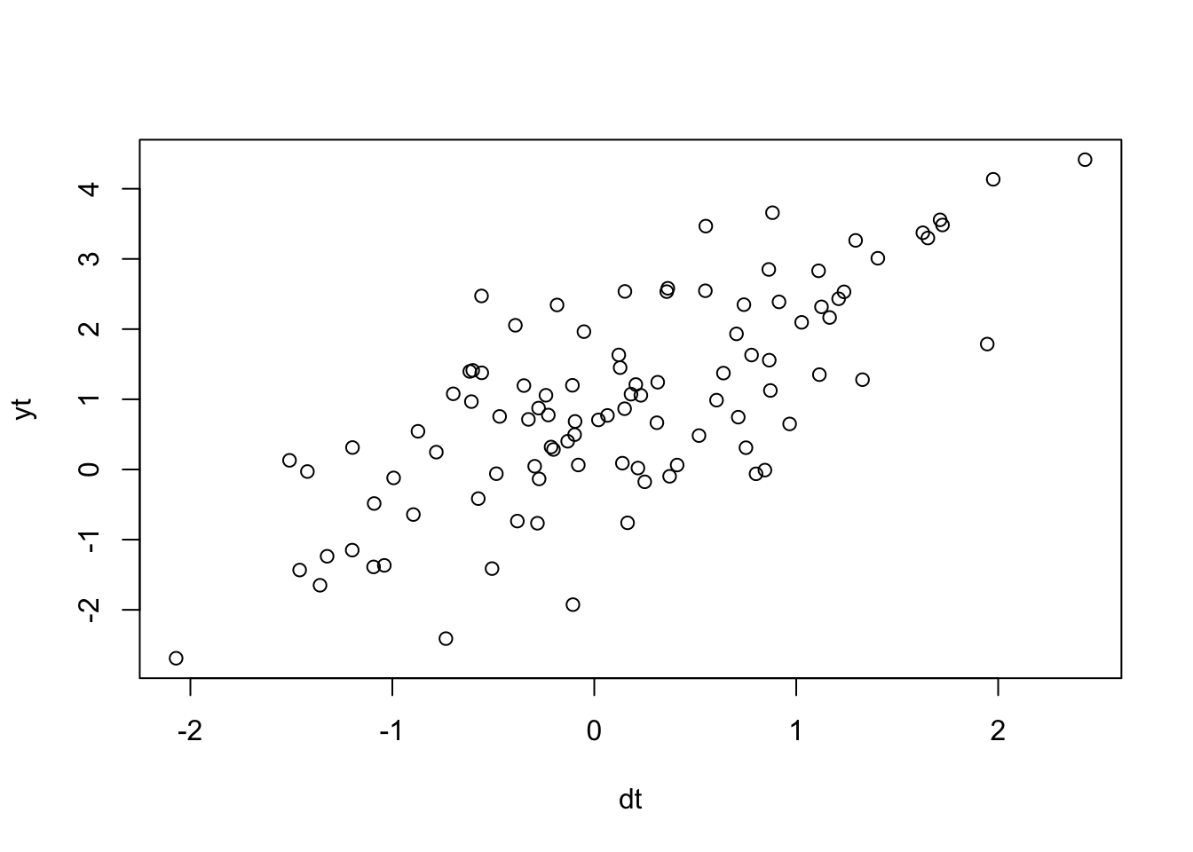
Let’s create some simulated data with this structure:

beta <- 1.1
alpha <- 1
r <- 1
dt <- rnorm(TT, 0, 1)  #our covariate
vt <- rnorm(TT, 0, r)
yt <- alpha + beta * dt + vt
plot(dt, yt)

To fit this model, we need to write it in MARSS form. Here’s the parts we need with the parameters, we don’t need removed. \(\mathbf{x}\) parameters to 0 so the algorithm doesn’t try to estimate them.

R <- matrix("r")  # no v_t
D <- matrix("beta")
d <- matrix(dt, nrow = 1)
Z <- matrix(0)
A <- matrix("alpha")
Q <- U <- x0 <- matrix(0)

MARSS() requires \(\mathbf{d}\) be a matrix also. Each row is a covariate and each column is a time step. No missing values allowed as this is an input.

mod.list <- list(U = U, Q = Q, x0 = x0, Z = Z, A = A, D = D, 
    d = d, R = R)
fit <- MARSS(yt, model = mod.list)

Success! algorithm run for 15 iterations. abstol and log-log tests passed.
Alert: conv.test.slope.tol is 0.5.
Test with smaller values (<0.1) to ensure convergence.

MARSS fit is
Estimation method: kem 
Convergence test: conv.test.slope.tol = 0.5, abstol = 0.001
Algorithm ran 15 (=minit) iterations and convergence was reached. 
Log-likelihood: -140.495 
AIC: 286.9899   AICc: 287.2399   
 
        Estimate
A.alpha    0.810
R.r        0.972
D.beta     1.227
Initial states (x0) defined at t=0

Standard errors have not been calculated. 
Use MARSSparamCIs to compute CIs and bias estimates.

The estimates are the same as with lm():

lm(yt ~ dt)

Call:
lm(formula = yt ~ dt)

Coefficients:
(Intercept)           dt  
     0.8096       1.2273